这是很早之前貌似从一本书上学习 Mathematica 时写的,算法原理也是书上的,年代太久远,我记不清楚出处了。
定义两个函数,分别是 CartesianMap 和 PolarMap 用来处理直角坐标和极坐标下的绘图,可接受绘图参数来控制图形显示效果。( 这两个函数后来加入系统扩展包中了,再到后来又取消了,见评论链接,不过仍然不失为一种不错的方法)具体用法我举几个例子说明一下。
$Lines = 15;
Options[CartesianMap] = Options[PolarMap] = {Lines -> $Lines};
CartesianMap[
    func_, {x0_, x1_, dx_: Automatic}, {y0_, y1_, dy_: Automatic},
    opts___?OptionQ] /;
   VectorQ[{x0, x1, y0, y1},
     NumericQ] && (NumericQ[dx] ||
      dx === Automatic) && (NumericQ[dy] || dy === Automatic) :=
  Module[{x, y},
   Picture[CartesianMap,
    func[x + I*y], {x, x0, x1, dx}, {y, y0, y1, dy}, opts]];
PolarMap[func_, {r0_: 0, r1_, dr_: Automatic}, {p0_, p1_,
     dp_: Automatic}, opts___?OptionQ] /;
   VectorQ[{r0, r1, p0, p1},
     NumericQ] && (NumericQ[dr] ||
      dr === Automatic) && (NumericQ[dp] || dp === Automatic) :=
  Module[{r, p},
   Picture[PolarMap,
    func[r*Exp[I*p]], {r, r0, r1, dr}, {p, p0, p1, dp}, opts]];
PolarMap[func_, rr_List, opts_?OptionQ] :=
  PolarMap[func, rr, {0, 2*Pi}, opts];
Picture[cmd_, e_, {s_, s0_, s1_, ds_}, {t_, t0_, t1_, dt_}, opts___] :=
   Module[{hg, vg, lines, nds = ds, ndt = dt},
   lines = Lines /. {opts} /. Options[cmd];
   If[Head[lines] =!= List, lines = {lines, lines}];
   If[ds === Automatic, nds = N[(s1 - s0)/(lines[[1]] - 1)]];
   If[dt === Automatic, ndt = N[(t1 - t0)/(lines[[2]] - 1)]];
   hg = Curves[e, {s, s0, s1, nds}, {t, t0, t1}, opts];
   vg = Curves[e, {t, t0, t1, ndt}, {s, s0, s1}, opts];
   Show[Graphics[Join[hg, vg]],
    Evaluate[FilterRules[{opts}, Options[Graphics]]],
    AspectRatio -> Automatic, Axes -> True]];
Curves[xy_, spread_, bounds_, opts___] :=
  With[{curves = Table[{Re[xy], Im[xy]}, spread]},
   ParametricPlot[curves, bounds, DisplayFunction -> Identity,
     Evaluate[FilterRules[{opts}, Options[ParametricPlot]]]][[1]]];
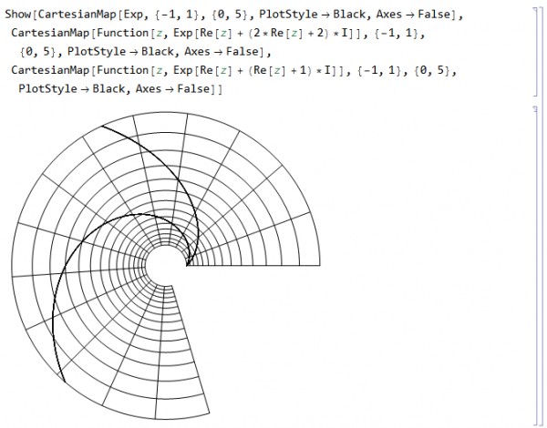
指数函数
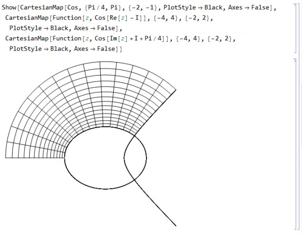
余弦函数
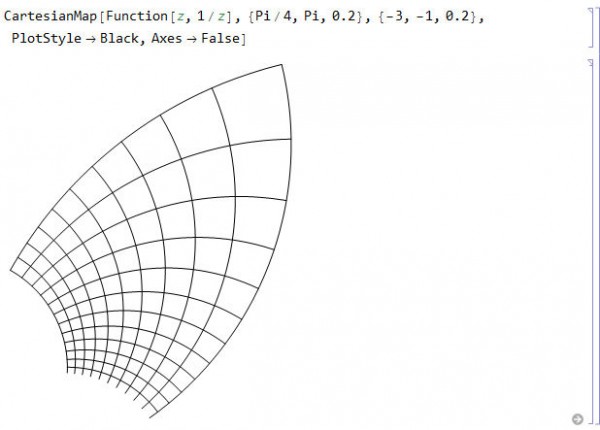
自定义的函数:倒数
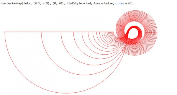
Zeta 函数
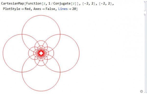
复共轭的倒数
上面都是直角坐标下的图形,极坐标下的用法是完全相同的,不再举例说明。

